Abstract
A leveraged index fund structure is presented that does not suffer from path dependence. As such, it is appropriate for long-term investment, including being suitable for retirement accounts.
1. Introduction
This article addresses a novel method of structuring leveraged index funds to remove their path dependence, making them suitable for long-term investment, including retirement accounts. The article describes the path dependency problem with current leveraged index funds and presents a solution that enables even conservative investors to avail themselves of leveraged returns while making long-term investments in such indices as the S&P500, the Dow Jones Industrial Average, or the NASDAQ. Because these indices are designed to continuously rise over the long term (because laggard companies are frequently removed and replaced by growth companies), long-term investors can be expected to obtain outsized returns without incurring outsized risk.
2. Background
Leveraged Index ETFs have been around for more than a decade. They enable speculators to invest in standard indices such as the S&P 500 and the Dow Jones Industrial Average and obtain returns that are multiples of the returns to their underlying index. Speculators can even bet against these indices by purchasing inverse funds that provide positive returns when their underlying index declines.
The way these funds work is based on the percentage change in the underlying index. If the index rises 2% on a particular day, a 2X leveraged index fund would rise 4%. A further benefit of this approach is that they can never go below zero. Since the underlying indices will always have a positive value, the most an index could decline is 99.99%. And realistically, such a dramatic loss in current leveraged index products such as the S&P500, Dow Jones Industrials, NASDAQ, etc. rarely see declines of more than 20%. This makes investing in such funds preferable to obtaining leverage by buying on margin, because there are no margin calls.
The promise of these funds – the ability to obtain leveraged returns on investments in traditional indices that historically rise over the long term without the risk of a margin call – prompted many investors to jump into them when they were first offered. But early investors – many of whom failed to read the prospectus for the ETF they purchased – were shocked by the disappointing results that they achieved.
3. The Problem
Exciting as the prospects of earning outsized returns when correctly judging whether the market will move up or down, all current leveraged index funds suffer from a shortcoming that is inherent in the way they are structured. They are all path dependent. What this means is that the value of the ETF loses fidelity with the underlying index after a short, predetermined period – typically one day for most US ETFs. This is the result of simple arithmetic.
For example, imagine a notional index is at 100 and a 2X ETF is also at 100 on the morning it is purchased. At the day’s closing bell, the index rises 10% to 110. The ETF would then rise 20% to 120 – a tidy gain. The next day, the index returns to 100 (a loss of ~9%). The ETF then declines just over 18%. But 18% of 120 is more the $20 ($21.8). The ETF is now below its initial purchase price (98.18) – even though the underlying index is exactly where it was when the investment began. There is no smoke and mirrors involved. It is just arithmetic. Over longer periods of time, particularly over periods of extreme volatility in the underlying index, this problem can grow.
This loss of fidelity over time means that if you purchase a 2x leveraged index ETF when the underlying index is at 100 and over several weeks the index rises to 110, the return on the investment will depend on the path the index took to get to 110. If it went up a bit every day until it reached 110, the return will actually exceed 2X. However, if the path from 100 to 110 was a volatile one with many dramatic ups and downs, the return will be less than 2X. In fact, in volatile periods (e.g., major market crashes) an investor could even lose money – even though he correctly guessed the direction of the market over the investment period. For example, during the financial crisis of 2008, if you purchased an inverse ETF, such as the ProShares UltraShort -2X ETF which is based on the Dow Jones Industrial Average on October 23, 2008, and sold it on March 4, 2009, the DJIA would have fallen 21% as shown in Table 1.
Table 1: Even though the DJIA lost 21%, the inverse, -2X ETF — rather than generating a handsome profit — generated a significant loss.
| DATE | DJIA | %change | DXD | %change |
| 23-Oct-08 | 8691.25 | 94.53 | ||
| 04-Mar-08 | 6875.84 | -21% | 79.00 | -16% |
At first blush one would expect that the investment in the DXD should yield a 42% profit for the five-month period. But, in fact the investment would have yielded a loss of 16% as shown in the table.
This was not a fault of ProShares. The same would have occurred with the other leveraged index funds on the market. The cause of this shocking result was the path dependence of all current leveraged ETFs. This path dependence limits investing in such instruments only to speculators. Because most current leveraged index ETFs in the US market re-index on a daily basis, they are best used for daily or intraday trading. They are not structured for a longer-term buy-and-hold strategy. This also tends to make them unsuitable for retirement accounts.
But wouldn’t it be great to be able to purchase a 2x ETF as part of a 401(k) account and watch it grow over one’s working career? Certainly, there might be pain some squeamishness during market downturns, but the major indices have always righted themselves and gone on to new highs. If only a fund could be structured that was not path dependent.
4. A Solution
Recognizing this problem, we were frustrated by the inability of the market to offer a leveraged index ETF that we could purchase as part of our 401(k) program. Accordingly, we set out to develop a fund structure that provided the benefits of leverage, that can be used in retirement accounts (i.e., without the risk of margin calls), that was not path dependent. And we succeeded! We call the resulting family of fund models ?Funds™.
If we made the same trade illustrated in Table 1 using an inverse 2X ?Fund™ we would obtain the results illustrated in Table 2.
Table 2: In contrast to the trade shwon in Table 1 using a traditional -2X leveraged index fund, rather than losing 16%, the -2X ?Fund™ obtains a nominal return of 42% — exactly what would be expected from its leverage.
| DATE | DJIA | Nominal change | %change | -2X ?Fund™ | Nominal change | %change |
| 23-Oct-08 | 8691.25 | 8691.25 | ||||
| 04-Mar-08 | 6875.84 | -1815.41 | -21% | 12322.07 | 3630.82 | 42% |
As can be seen from the table, the return of the ?Fund™ structure is 42% — in line with expectations of a -2X leveraged fund given the change in the underlying index of -21%. This stands in marked contrast to the performance of traditional -2 leveraged funds which lost money during this period. (Actual returns would be slightly less because of the fund manager’s fees, but even with a high fee of 2% per year, the profit would be quite healthy.
Not being fund managers, ourselves, there is not yet an implementation of this fund structure. But we have extensively modeled our fund structure and back-tested it under all market conditions for both the S&P500 and the DJI going back several decades. The fund performed as expected: if the market was up, the fund was up; if the market was down, the fund was down; and when the index was neutral, the fund was neutral. We performed tests under all market conditions through the Great Depression, the Internet Bubble, the 2008 mortgage crisis, and all markets in between.
We show the results of both 2X and -2X ?Funds™ based on the S&P500 in Table 3. Table 3 measures performance of an investment made on the first trading day of the volatile year of 2008: January 2. We took measurements on the first trading day of each subsequent month.
Table 3: An example investment in both a 2X ?Fund™ and a -2X ?Fund™ based on the S&P500 for the volatile year of 2008 shows that both retain fidelity with the underlying S&P500 index throughout the year.
| S&P500 Index | 2X ?Fund™ | -2X ?Fund™ | |||||||
| DATE | S&P500 | Nominal change | Cumulative % return | 2X ?Fund™ | Nominal change | Cumulative % return | -2X ?Fund™ | Nominal change | Cumulative % return |
| Jan-08 | 1447.16 | 1447.16 | 1447.16 | ||||||
| Feb-08 | 1395.42 | -51.74 | -3.6% | 1343.68 | -103.48 | -7.2% | 1550.64 | 103.48 | 7.2% |
| Mar-08 | 1331.34 | -64.08 | -8.0% | 1215.52 | -128.16 | -16.0% | 1678.80 | 128.16 | 16.0% |
| Apr-08 | 1370.18 | 38.84 | -5.3% | 1293.20 | 77.68 | -10.6% | 1601.12 | -77.68 | 10.6% |
| May-08 | 1409.34 | 39.16 | -2.6% | 1371.52 | 78.32 | -5.2% | 1522.80 | -78.32 | 5.2% |
| Jun-08 | 1385.67 | -23.67 | -4.2% | 1324.18 | -47.34 | -8.5% | 1570.14 | 47.34 | 8.5% |
| Jul-08 | 1284.91 | -100.76 | -11.2% | 1122.66 | -201.52 | -22.4% | 1771.66 | 201.52 | 22.4% |
| Aug-08 | 1260.31 | -24.60 | -12.9% | 1073.46 | -49.20 | -25.8% | 1820.86 | 49.20 | 25.8% |
| Sep-08 | 1277.58 | 17.27 | -11.7% | 1108.00 | 34.54 | -23.4% | 1786.32 | -34.54 | 23.4% |
| Oct-08 | 1161.06 | -116.52 | -19.8% | 874.96 | -233.04 | -39.5% | 2019.36 | 233.04 | 39.5% |
| Nov-08 | 966.30 | -194.76 | -33.2% | 485.44 | -389.52 | -66.5% | 2408.88 | 389.52 | 66.5% |
| Dec-08 | 816.21 | -150.09 | -43.6% | 185.26 | -300.18 | -87.2% | 2709.06 | 300.18 | 87.2% |
To make comparisons easy, we gave the fund the same value as the closing price of the S&P500 on this day. This may be a bit misleading, because only in this scenario will percentage returns be the same as the nominal returns upon which the fund model is based. Investing at any other time, the cumulative percentage returns will not be exactly 2X or -2X. But it will still be the case that:
- If the index is up, the fund will be up.
- If the index is down, the fund will be down.
- If the index is neutral the fund will be neutral.
At no time will a favorable change in the underlying index result in an unfavorable outcome.
To illustrate this divergence in the percentage return, we show the same investment depicted in Table 4. Instead of buying the fund on January 2, we illustrate the impact of making the investment on March 3.
Table 4: Making an investment on any day after the fund is initiated will cause the amount of leverage to vary. The cumulative percentage return will not be an exact multiple of the leverage factor times the return of the index. But the direction of the return (e.g., profit or loss) continues to maintain fidelity with the underlying index.
| S&P500 Index | 2X ?Fund™ | -2X ?Fund™ | |||||||
| DATE | S&P500 | Nominal change | Cumulative % return | 2X ?Fund™ | Nominal change | Cumulative % return | -2X ?Fund™ | Nominal change | Cumulative % return |
| Jan-08 | 1447.16 | 1447.16 | 1447.16 | ||||||
| Feb-08 | 1395.42 | -51.74 | 1343.68 | -103.48 | 1550.64 | 103.48 | |||
| Mar-08 | 1331.34 | -64.08 | 1215.52 | -128.16 | 1678.80 | 128.16 | |||
| Apr-08 | 1370.18 | 38.84 | 2.9% | 1293.20 | 77.68 | 6.4% | 1601.12 | -77.68 | -4.6% |
| May-08 | 1409.34 | 39.16 | 5.9% | 1371.52 | 78.32 | 12.8% | 1522.80 | -78.32 | -9.3% |
| Jun-08 | 1385.67 | -23.67 | 4.1% | 1324.18 | -47.34 | 8.9% | 1570.14 | 47.34 | -6.5% |
| Jul-08 | 1284.91 | -100.76 | -3.5% | 1122.66 | -201.52 | -7.6% | 1771.66 | 201.52 | 5.5% |
| Aug-08 | 1260.31 | -24.60 | -5.3% | 1073.46 | -49.2 | -11.7% | 1820.86 | 49.20 | 8.5% |
| Sep-08 | 1277.58 | 17.27 | -4.0% | 1108.00 | 34.54 | -8.8% | 1786.32 | -34.54 | 6.4% |
| Oct-08 | 1161.06 | -116.52 | -12.8% | 874.96 | -233.04 | -28.0% | 2019.36 | 233.04 | 20.3% |
| Nov-08 | 966.30 | -194.76 | -27.4% | 485.44 | -389.52 | -60.1% | 2408.88 | 389.52 | 43.5% |
| Dec-08 | 816.21 | -150.09 | -38.7% | 185.26 | -300.18 | -84.8% | 2709.06 | 300.18 | 61.4% |
Our structure obviously differs from the current structure. To avoid path dependence, we apply leverage to the nominal change in an index, not its percentage change. In this way, when the index is at a particular value X, the ETF would have a value Y. And even if the market goes through a major crisis, when the index returns to X, the ETF will have the exact value Y. There is a 1:1 correspondence of the ETF value to the underlying index for every value of the index. But the leverage will diminish as the fund value rises and it will increase as the fund value declines. And unlike current funds, when the index retraces itself, the ?Fund™ leverage will also retrace itself, enabling the fund to exactly retrace its value. In this way, for any given value of the underlying index, the value of the fund will always be the same. Looking at Table 4 and the values on September 8, 2008, the S&P500 closed at 1277.58 and the 2X ?Fund™ closed at 874.96. When the S&P eventually recovered to the 1277.58 level intraday in January 2011, the ?Fund™ would also recover to exactly 874.96.
As can be seen in Table 4, the cumulative return percentages of the 2X ?Fund™ are no longer exact multiples of the cumulative return of the underlying index. But they continue to reflect leveraged returns in the expected direction. This is because the 2X ?Fund™ was purchased at a price below the initial offering price. As such the nominal change in the 2X fund will be a greater percentage of the purchase price ($1215.52) than had it been purchased at the initial opening price ($1447.16). Therefore, on December 8, the leverage of the 2X ?Fund™ was 2.2. Once purchased, however, the leverage does not change for the life of the investment. The leverage is merely a function of using a different denominator (the purchase price) versus the initial offering price.
For the inverse fund, the inverse logic applies. Purchased at a higher price ($1678.80) than the initial offering price ($1447.16), the leverage on the -2X ?Fund™ declined to 1.6.
Because, in general, indices such as the S&P500 rise over time, it can be expected that a positive leverage (e.g., 2X of 3X) will experience significant losses of leverage over time. The leverage will always be present, but at levels just above 1.0, the appeal of the fund to investors could diminish. A way for a fund manager to address this would be to issue a new fund beginning at the higher current value. Investors could then take profits in the positions in the old fund and invest in the new one to maintain higher levels of leverage.
To view a longer-term investment we capture an investment beginning in January, 2008, and display the value of a 2X leveraged ?Fund™ for the first trading day of every succeeding year in Table 5.
Table 5: A long-term investment in 2X leverage ?Fund™, based on the S&P500 would yield a return double that of the underlying S&P500 Index (before the reduction of fund management fees).
| S&P500 Index | 2X ?Fund™ | |||||||
| DATE | S&P500 | Nominal change | Cumulative % return | 2X ?Fund™ | Nominal change | Cumulative % return | ||
| 2008-01-02 | 1447.16 | 1447.16 | ||||||
| 2009-01-02 | 931.80 | -515.36 | -35.6% | 416.44 | -1030.72 | -71.2% | ||
| 2010-01-04 | 1132.99 | 201.19 | -21.7% | 818.82 | 402.38 | -43.4% | ||
| 2011-01-03 | 1271.87 | 138.88 | -12.1% | 1096.58 | 277.76 | -24.2% | ||
| 2012-01-03 | 1277.06 | 5.19 | -11.8% | 1106.96 | 10.38 | -23.5% | ||
| 2013-01-02 | 1462.42 | 185.36 | 1.1% | 1477.68 | 370.72 | 2.1% | ||
| 2014-01-02 | 1831.98 | 369.56 | 26.6% | 2216.80 | 739.12 | 53.2% | ||
| 2015-01-02 | 2058.20 | 226.22 | 42.2% | 2669.24 | 452.44 | 84.4% | ||
| 2016-01-04 | 2012.66 | -45.54 | 39.1% | 2578.16 | -91.08 | 78.2% | ||
| 2017-01-03 | 2257.83 | 245.17 | 56.0% | 3068.50 | 490.34 | 112.0% | ||
| 2018-01-02 | 2695.81 | 437.98 | 86.3% | 3944.46 | 875.96 | 172.6% | ||
| 2019-01-02 | 2510.03 | -185.78 | 73.4% | 3572.90 | -371.56 | 146.9% | ||
| 2020-01-02 | 3257.85 | 747.82 | 125.1% | 5068.54 | 1495.64 | 250.2% | ||
| 2021-01-04 | 3700.65 | 442.80 | 155.7% | 5954.14 | 885.60 | 311.4% | ||
| 2022-01-03 | 4796.56 | 1095.91 | 231.4% | 8145.96 | 2191.82 | 462.9% | ||
| 2023-01-03 | 3824.14 | -972.42 | 164.3% | 6201.12 | -1944.84 | 328.5% | ||
As can be seen from Table 5, the ?Fund™ purchased at the initiation of a ?Fund™ on January 2, 2008 would double both the nominal and percentage return on the purchase of a basic index fund. This is illustrated graphically in Figure 1.
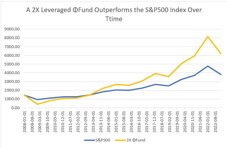
Figure 1: Because the 2X leveraged Fund maintains fidelity with its underlying index, it can be expected to provide outsized returns for underlying indices that always rise over time such as the S&P500 and the Dow Jones Industrial Average.
Purchases made at any time other than fund initiation would still produce outsized returns as shown in Table 6.
Table 6: Because the returns of the leveraged Fund are not path dependent, they maintain fidelity with the underlying index eternally. No re-indexing is ever required.
| S&P500 Index | 2X ?Fund™ | |||||
| DATE | S&P500 | Nominal change | Cumulative % return | 2X ?Fund™ | Nominal change | Cumulative % return |
| 2008-01-02 | 1447.16 | 1447.16 | ||||
| 2008-03-03 | 1331.34 | -115.82 | 1215.52 | -231.64 | ||
| 2009-01-02 | 931.80 | -399.54 | -30.0% | 416.44 | -799.08 | -65.7% |
| 2010-01-04 | 1132.99 | 201.19 | -14.9% | 818.82 | 402.38 | -32.6% |
| 2011-01-03 | 1271.87 | 138.88 | -4.5% | 1096.58 | 277.76 | -9.8% |
| 2012-01-03 | 1277.06 | 5.19 | -4.1% | 1106.96 | 10.38 | -8.9% |
| 2013-01-02 | 1462.42 | 185.36 | 9.8% | 1477.68 | 370.72 | 21.6% |
| 2014-01-02 | 1831.98 | 369.56 | 37.6% | 2216.80 | 739.12 | 82.4% |
| 2015-01-02 | 2058.20 | 226.22 | 54.6% | 2669.24 | 452.44 | 119.6% |
| 2016-01-04 | 2012.66 | -45.54 | 51.2% | 2578.16 | -91.08 | 112.1% |
| 2017-01-03 | 2257.83 | 245.17 | 69.6% | 3068.50 | 490.34 | 152.4% |
| 2018-01-02 | 2695.81 | 437.98 | 102.5% | 3944.46 | 875.96 | 224.5% |
| 2019-01-02 | 2510.03 | -185.78 | 88.5% | 3572.90 | -371.56 | 193.9% |
| 2020-01-02 | 3257.85 | 747.82 | 144.7% | 5068.54 | 1495.64 | 317.0% |
| 2021-01-04 | 3700.65 | 442.80 | 178.0% | 5954.14 | 885.60 | 389.8% |
| 2022-01-03 | 4796.56 | 1095.91 | 260.3% | 8145.96 | 2191.82 | 570.2% |
| 2023-01-03 | 3824.14 | -972.42 | 187.2% | 6201.12 | -1944.84 | 410.2% |
Table 6 assumes the same purchase date of March 3, 2008 as shown in Table 4. Because the purchase price ($1215.52) was lower than the initial purchase price ($1447.16), the returns of the fund reflect a 2.2X leverage, returning over 400% over the nearly 15-year period, versus the 187% return of the S&P500 (both exclusive of management fees).
4.1. Solving a minor glitch
Using the nominal value, rather than a percentage value could have the potential to cause the fund value to go negative. If an index begins at 100 and a -2X ?Fund™ also begins at 100 and the index rises 51 points to 151, the -2X ?Fund™ should decline 102 points which would give it an unacceptable valuation of -2. We resolve this by creating a tapering of the leverage below a fixed threshold. If the threshold is reached, the leverage declines. Using zero as an asymptote, the leverage changes continuously so that a zero valuation is never attained. Equally important, if/when the fund value begins to rise the leverage follows the identical path on its way up. In this way, there remains a 1:1 correlation of the value of the fund to the value of the underlying index. In fact, the values of the fund can be published to show the value of the fund for any value of the underlying index. And because it is not path dependent, the values will remain constant over all periods of time.
Our work has received US patent US 8,296,214. It has also been granted in several other major world markets.
5. Conclusion
It is possible to create a leveraged index ETF that maintains fidelity with its underlying index under all market conditions for all time frames. The resulting fund is not path dependent and is suitable for long-term portfolios including retirement accounts. If the fund is based on an index that is designed to rise over time (e.g., the S&P500 and the Dow Jones Industrial Average), a leveraged ?Fund™ can be expected to consistently provide outsized returns over the period of a long-term investment using a buy-and-hold strategy. It, therefore, would be suitable for a retirement account, such as a 401(k), if the account owner still anticipated many more years of life.
6. Bibliography
Elisabeth Kashner, “The Truth About Leveraged ETF Returns”, https://www.etf.com/sections/blog/21176-the-truth-about-leveraged-etf-returns.html, February 11, 2014.
Marco Avellaneda and Stanley Zhang, “Path-Dependence of Leveraged ETF Returns” SIAM Journal on Financial MathematicsVol. 1, Iss. 1 (2010)10.1137/090760805, https://math.nyu.edu/~avellane/SIAMLETFS.pdf.pdf, 2010.
Jian Zhang, “Path-dependence properties of leveraged exchange-traded funds: Compounding, volatility and option pricing”, https://www.semanticscholar.org/paper/Path-dependence-properties-of-leveraged-funds%3A-and-Zhang/08a74f6420b644985fd2737066f0ba51acb6ae95, 2010.
Jeff Stollman, “In Search of Leveraged Returns for Long-term Investment”, http://www.phi-funds.com/2015/05/19/in-search-of-leveraged-returns-for-long-term-investment/, May 19, 2015.